3. Fancy interplanetary OSPREI
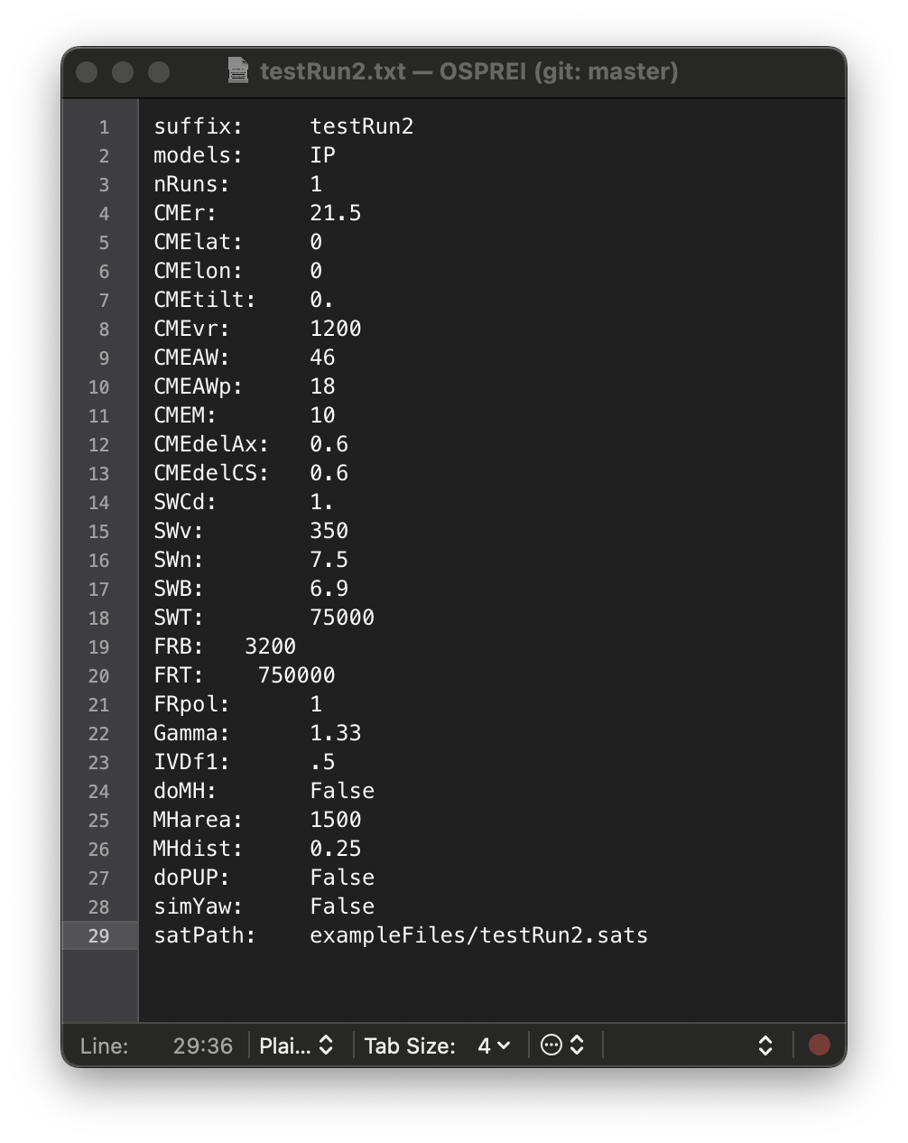 Open testRun2.txt and notice that now we have a lot more input options than before. The first group of these are solar wind (SW) parameters. These are the values at the satellite location, which are then used to scale a simple 1D empirical background SW, and the drag coefficient, Cd. If the satellite is near 1 AU then OSPREI will default to average values, which is what happened in our first example. The SW numbers in this .txt file are the same as the default values so the CME behavior should be the same as the previous case (up to some small rounding errors due to precision of inputs/defaults). We have a few additional parameters, Gamma and IVDf1. Gamma controls the adiabatic index of the CME and how the expansion affects the internal temperature. The initial velocity decomposition sets the initial CME expansion relative to the propagation speed. It can be set anywhere between 0 and 1, which correspond to the limits of self-similar expansion (0) or purely convective flow (1). For basic use these can be left at the default values of 1.33 (ideal monatomic gas) and 0.5 (halfway between self similar and convective).
The rest of the additions represent adding major components to the model operations, which we will discuss below. The other major change is in the satellite properties. Instead of a the list of parameters in the first test run, we now use satPath to point to a satellite path file. We label these files ".sats" (or ".sat") but they are just normal plain text files. testRun2.sats contains 9 lines, each of which has a satellite name, latitude (°), longitude (°), radial distance (Rs), and orbital speed (rad/s). We have set up a string of stationary satellites separate by 10° in longitude. OSPREI can run a single CME simulation but produce results for up to 10 satellites simultaneously. Due to some unique python "features" with lambda functions we have a upper limit of 10 satellites, which should be sufficient for any reasonable cases, but reach out if you need to add more (or just run OSPREI multiple times with different satellite files)
Run OSPREI with this second test run before we turn on any of the fancier features. The beginning is the same as before but once it starts impacting satellites we get a longer list of the satellite impact details at each time step.
 48.52 193.53 492.60  54.52  27.41   0.30   0.28   7.85   4.83 106.03   0.00   0.00   0.00
       Sat4  0.95879 64.80005 -0.08219
       Sat4n  0.95879 -64.80005 -0.08219
 48.53 193.57 492.55  54.52  27.42   0.30   0.28   7.85   4.83 106.00   0.00   0.00   0.00
       Sat4  0.95677 64.80005 -0.07064
       Sat4n  0.95677 -64.80005 -0.07064
 48.57 193.66 492.45  54.52  27.42   0.30   0.28   7.84   4.83 105.94   0.00   0.00   0.00
       Sat4  0.95274 64.80005 -0.04741
       Sat4n  0.95274 -64.80005 -0.04741
It first impacts the satellites at ±40° as our initial configuration causes the CME to pancake so the edges are at a slightly farther radial distance than the CME nose. Eventually it passes over all the satellites then returns the impact time information for each satellite at the bottom. Run processOSPREI on this case. The same three types of figures will appear in the NoDate folder. There is still a single DragLess figure, but there is a J Map and IS figure for each satellite.
3.1 CME-Driven Sheath
Now we move on to additional features that can be included within the interplanetary part of the simulation. Switch doPUP to True. This includes the Pile Up Procedure to add a CME-driven sheath. Rerun the simulation. It will run a little slower than before since we are now solving the MHD shock/jump conditions to determine the compression upstream of the CME. At each time step we now have an additional line printing to the screen, giving information about the sheath.
    0.02  21.60 1198.73  46.00  18.00   0.60   0.60 11653.18   5.87 5300.31   0.00   0.00   0.00
        3.77 1506.64   3.21   0.03   0.00   0.01 2743.57   7.19 522.63   0.00
  0.17  22.52 1188.07  46.00  18.00   0.59   0.59 10318.55   5.86 5015.48   0.00   0.00   0.00
        3.78 1491.49   3.31   0.26   0.04   0.09 2481.80   7.18 481.44   0.00
  0.33  23.54 1177.69  46.01  18.01   0.59   0.58 9068.68   5.84 4722.08   0.00   0.00   0.00
        3.78 1476.64   3.42   0.52   0.09   0.18 2234.20   7.17 441.92   0.00
  0.50  24.54 1168.54  46.02  18.03   0.58   0.57 8013.39   5.82 4449.45   0.00   0.00   0.00
        3.79 1463.53   3.53   0.77   0.13   0.27 2022.84   7.16 407.74   0.00
The top line is the same CME information as before. The second line (indented) shows the sheath compression, shock speed (km/s), Alfvenic Mach number, sheath width (Rs), duration (hr), mass (1015 g), density (cm-3), log(T) (K), B, and a flag for when the satellite first enters the sheath (0→1). The satellite line will now also print when the CME is within the sheath, which will show a fractional radial distance greater than 1. The final output for this case should be (showing only results for Sat0):
Satellite:         Sat0
Transit Time:      48.53333333333333
Final Velocity:    601.6716576955699 67.46515806469739
CME nose dist:     213.0172256177004
Sat. longitude:    0.0
Est. Duration:     25.200000000000003


0 Contact after 2.02 days with front velocity 601.67 km/s (expansion velocity 67.47 km/s) when nose reaches 213.02 Rsun and angular width 53 deg and estimated duration 25 hr
   Density:  6.442479966288627   Temp:   62825.20497441381
We see that the CME ends up propagating a bit faster than in the sheath-less case. Note that the sentence is still printing the time of first contact with the flux rope, not first contact with the sheath, so the flux rope does actually arrive quicker. The model includes the extra mass of the swept-up sheath in the drag propagation, reducing the effectiveness of the drag force in decelerating the CME.
We now have additional files in NoDate labeled PUPresultstestRun2.dat and SITresultstestRun2SatX.dat, where X represents each of the satellite names. PUPresultsdemo.dat contains the actual evolution of the sheath with IP distance and the SITresultstestRun2SatX.dat file contains a single line with properties at first contact at that satellite (this is more useful for ensemble cases). The details of what each column represents within these files are in the appendix.
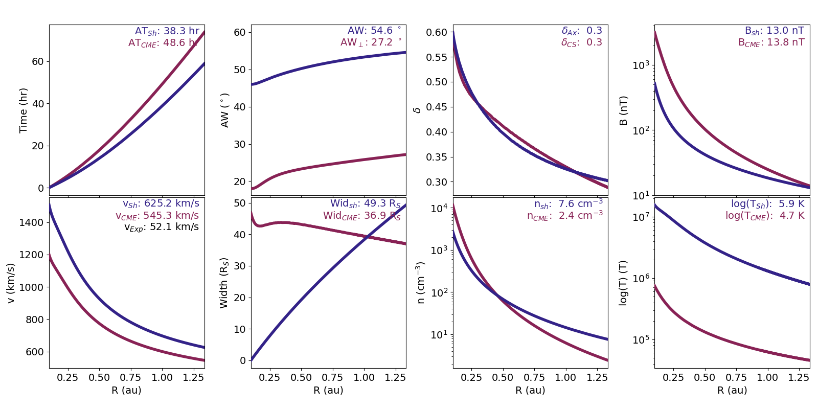
Run processOSPREI.py for the new results. We now get the same figures as before plus a new one fig_testRun2_ANTPUP.png. The ANTPUP figure is very similar to DragLess, but has more panels. In most panels, the maroon line represents the sheath and the blue one the CME/FR. The only exceptions are in the AW and δ panels where blue is face-on/axial and maroon is edge-on/cross-sectional.
The DragLess figure (not shown) is the exact same format as before but the precise behavior of each line changes due to the inclusion of the CME-driven sheath.
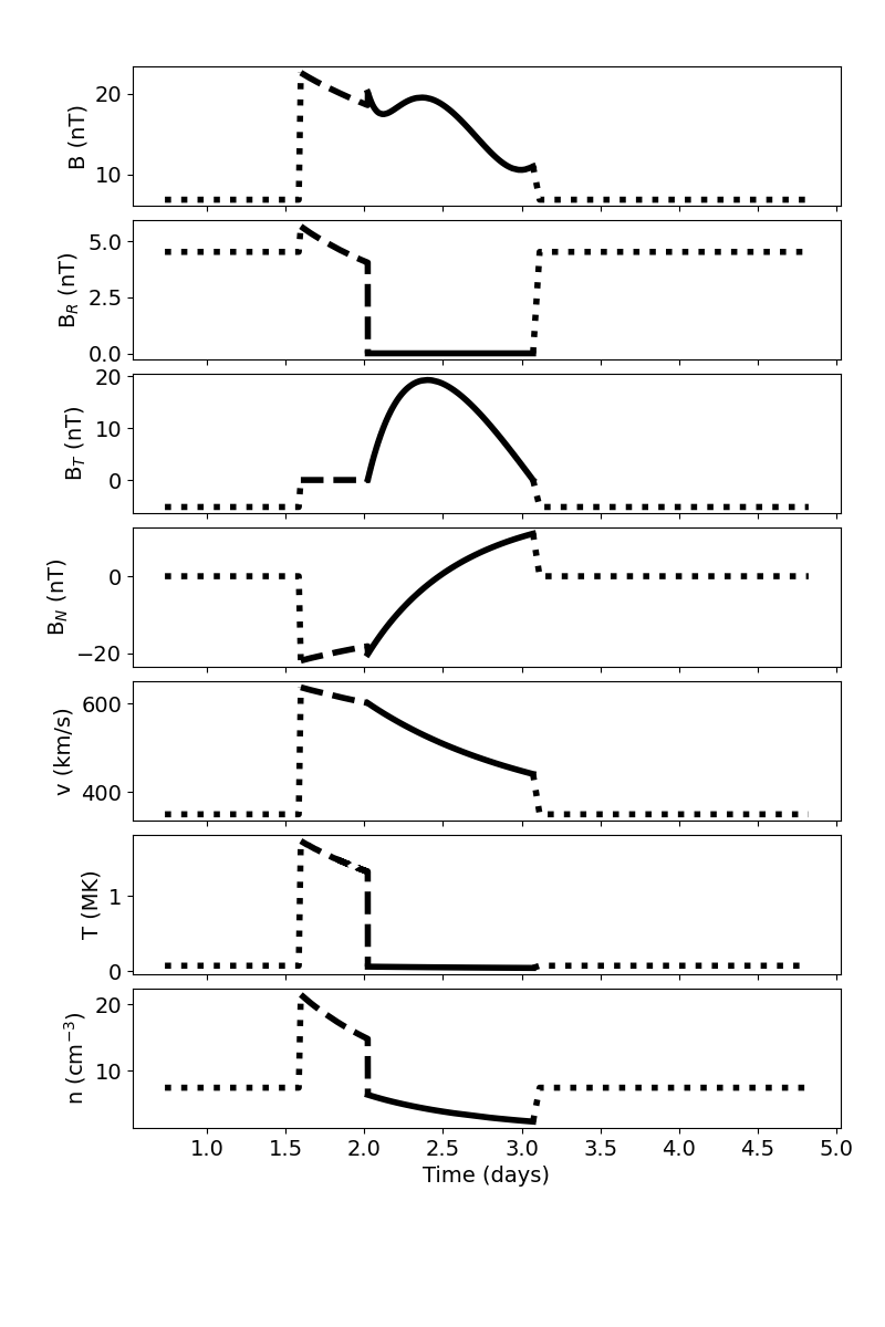 The in situ plot is similar to the previous version but the contents have slightly changed. We show the version for Sat0, which is for the same satellite location as testRun1. Now, in front of the solid line that represents the flux rope profile, we also see the sheath represented with a dashed line. OSPREI only models the average behavior within the highly turbulent sheath, we cannot include any of the stochastic fluctuations expected in a real event. The profiles do show how the upstream solar wind is compressed within the sheath region, causing enhancements in the magnetic field, temperature, and density.
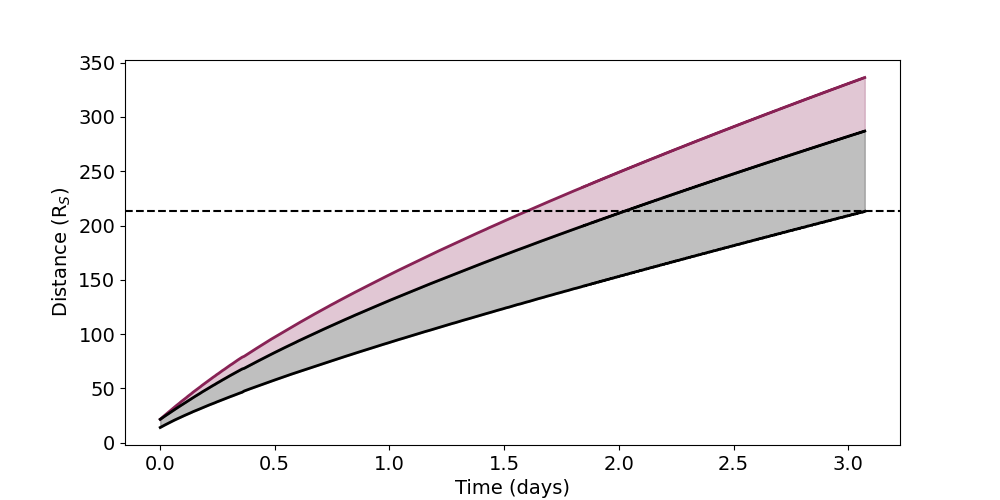 The J map figure is also similar to before, but now we see the maroon region representing the sheath ahead of the CME. The figure shows that both the sheath and flux rope grow in radial with over time.
Try playing with the CME and SW parameters and see how the sheath changes. Note that if the CME velocity is slower than the background SW then no sheath will form. The code should still run, but it will not accumulate material into the sheath unless the CME velocity begins exceeding the background velocity.
3.2 Background HSS
The next major component to try is a time-dependent high speed stream (HSS) background. This is the MEOW-HiSS model that was specifically developed to couple with OSPREI. It is essentially a set of simple empirical functions/coefficients that reproduce the results of MHD simulations. It was meant to be an adequate background for CME simulations but seems to have legitimate merit as a SW forecasting tool in its own right. More details, including how to find the appropriate CH area and HSS front distance for observed cases, can be found in the paper and there is an example of its use on the How to MEOW-HiSS page. Note that MEOW-HiSS adds in a HSS by scaling the simple, quiescent background (i.e. setting the velocity to be 2x the quiescent value at a given spot rather than explicitly setting it at 700 km/s) so all the quiescent SW input parameters still have an effect on the background.
Set doMH to True within testRun2.txt. The input file already has MHarea and MHdist set (units of 108 km2 and AU) and OSPREI was happily ignoring them while MEOW-HiSS was turned off. Run OSPREI again, there shouldn’t be a significant change in run time. Notice that in the output printed to the screen, the last number in the CME row begins at 4 then ends at 0. This is indicating which region the front of the CME is in at each time. The CME starts in the plateau of the HSS (4) and moves fast enough to go through the SIR (regs 3-1) then reach the quiescent SW upstream (0). We see a large change in the simulation results (showing only Sat0, the first line):
0 Contact after 1.70 days with front velocity 687.76 km/s (expansion velocity 33.13 km/s) when nose reaches 213.02 Rsun and angular width 50 deg and estimated duration 15 hr
Density: 9.265794036577446 Temp: 70830.06997439543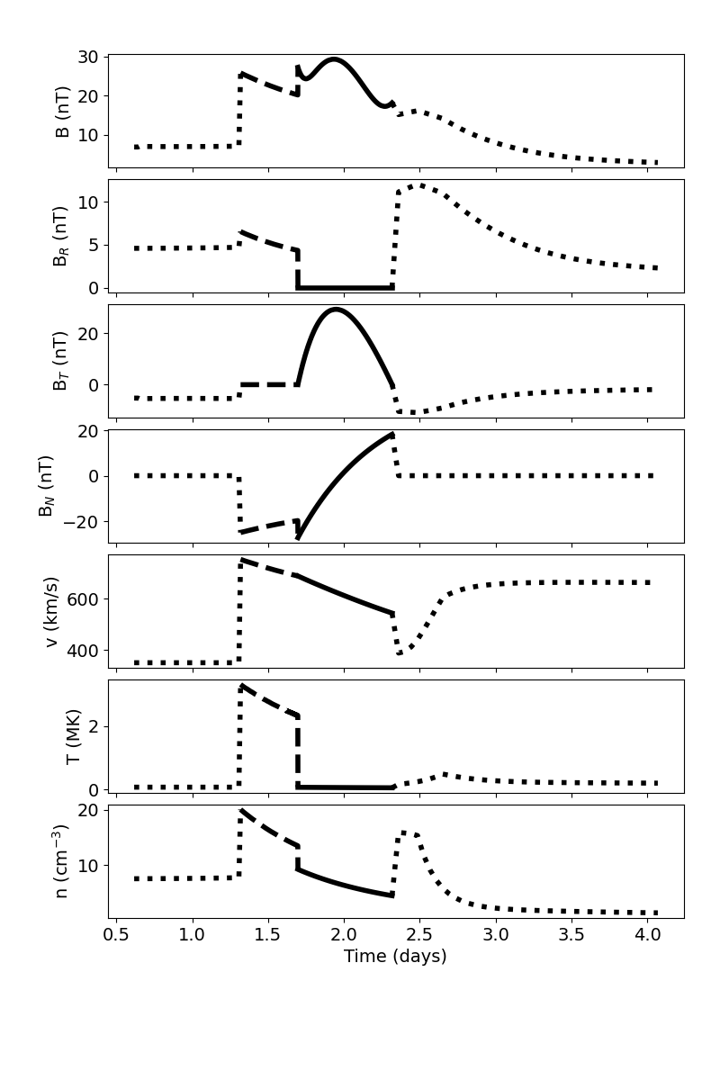 The faster SW background causes there to be significantly less drag and a faster CME at the time of arrival. Run processOSPREI.py. The in situ results have the same format as the previous iteration, but you can now see the CME is embedded in front of a HSS (most noticeable in the velocity panel). The in situ FR is more compressed and arrives earlier than the case in the quiescent background.
Open up processOSPREI.py. Line 44 (or hopefully somewhere near if there have been minor edits in the code but not the guide) sets doMovie to False. This turns off a fancy plotting procedure dubbed “enlilesque” that makes a Enlil-like set of images for the simulation. It runs a little slow so we default to not including it. Switch doMovie to True and run processOSPREI.py again. There will be a short delay as it runs the three plots we have been generating previously, then it will start counting as it makes Enlilesque figures. It produces a 2D contour for every 5 Rs of CME propagation (i.e. CME nose at 20 Rs, 25 Rs, …). This will continue running until the end of the simulation data. You can exit out of it using control+c to kill the running process.
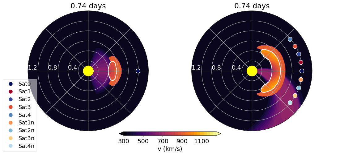
This generates a series of .png named fig_testRun2_Enlilesque###.png where the number is sequentially increasing. Below is number 020 as example. The figure shows contours of the velocity in the meridional and equatorial planes. The meridional plane is taken through the CME nose. The pale blue dot is the satellite and the CME is outlined in white. The velocity contours show the sheath ahead of the CME and the HSS. At this point we must emphasize that this is a only a clever visualization of our analytic/empircal model as we can project our results onto different planes in space, but we do not have a full 3D simulation with plasma properties consistently evolved across adjactent cells. We plot the HSS (making an approximation of its meridional width) and simply replace the HSS values with CME/sheath values wherever they overlap. With that in mind, it can be a useful visualization of the geometry of the interaction. In the call to enlilesque (line 283) you can toggle whether to plot the satellite, which planes to include (both, mer, or eq), and the limits of the contours (vel0 and vel1). You can also convert the series of images into a movie using additional software (I tend to use ImageMagick).
Play with MHarea and MHdist to get a sense of how the HSS affects the CMEs IP evolution. These parameters should be kept within [300, 2500] and [-0.4, 1.5]. We do allow negative distances for the HSS front, this corresponds to a HSS from a CH that has yet to rotate to the longitude at which the CME eruption occurs.
3.3 IP Rotation
The next feature is a rotation of the CME in IP space. If the CME flanks experience different amount of drag then one flank should move faster than the other, which will create a rotation. This feature is brand new, the paper was published in late 2023. That work finds that this rotation is typically quite small (usually less than 5°) but it can make a ~5 hour difference in arrival times.
Set simYaw to True to include this rotation and run OSPREI again. The final lines of the results become (again showing only the sat0 results):
5 59.15 274.14 609.45  51.80  26.20   0.32   0.21   3.88   4.73  99.31  10.35   0.03   0.00
        3.64 707.65   7.23  50.55  16.13  21.88   7.35   6.14  14.55   1.00

Satellite:         Sat0
Transit Time:      40.71666666666667
Final Velocity:    687.755536566486 33.130943953102296
CME nose dist:     213.01958780073323
Sat. longitude:    0.0
Est. Duration:     15.25

0 Contact after 1.70 days with front velocity 687.76 km/s (expansion velocity 33.13 km/s) when nose reaches 213.02 Rsun and angular width 50 deg and estimated duration 15 hr
   Density:  9.265794036577446   Temp:   70830.06997439543
The third to last column in the CME line of the printed output shows this “yaw” rotation (10.35 in the example) and the second to last column is the rotational velocity (in deg/hr). A yaw rotation is technically about the center of mass, rather than the CME nose as done in OSPREI for computational reasons, but we refer to it as such for simplicity. This CME actually rotates 10.35° by the time the satellite exits the CME, one of the largest rotations seen in OSPREI. This is because the inputs have been set to maximize the rotation. If you look at the enlilesque figure from section 3.2 you can see that one flank of the CME is embedded in the HSS and the other in the quiescent SW.
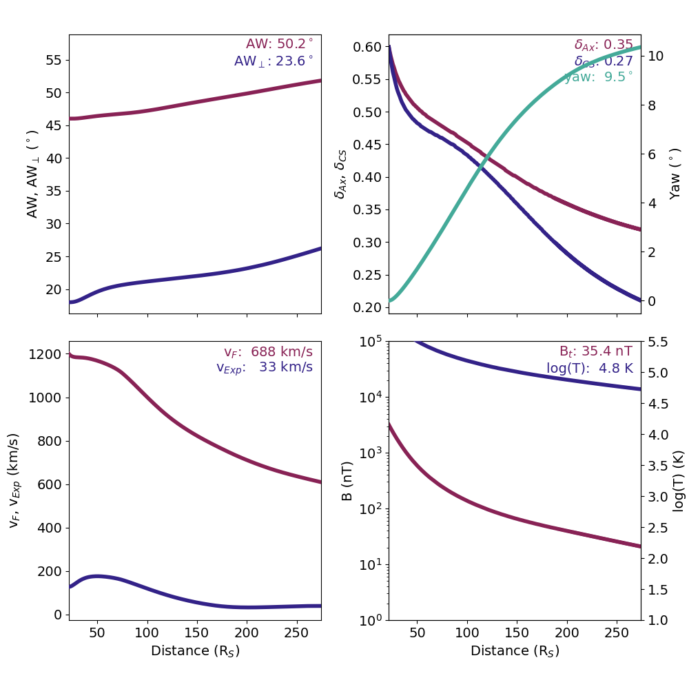 The transit time and other final properties are nearly the same at sat0 when we did not include rotation (in section 3.2) since this impact occurs directly at the CME nose. Comparing values towards the flanks leads to more noticeable varations. Run processOSPREI. Remember to switch the True back to a False at the bottom of processOSPREI.py if you do not want to keep making enlilesque figures. Look at the Drag figure you will see that the aspect ratio panel (top right) now also includes the yaw rotation in teal. The printed number is the value at the time at first contact, not the end of the simuation.
3.4 Real Cases and Fancy Satellites
Before moving onto full OSPREI runs, we look at interplanetary simulations of a real event. This is what one would do if you want to start from measurements of a CME in the outer corona rather than trying to simulate the full evolution from the initial eruption on the Sun. testRun3.txt demos this configuration for an eruption on 2023 Sep 23 that encountered four different spacecraft. OSPREI runs of this events were featured in Palmerio et al. 2024 but the testing input parameters are not the exact same as in the paper so the outputs will not be an exact match. We have turned on the CME-driven sheath but do not include any background HSS or yaw rotation in this example.
If you look at testRun3.sats you will see four lines in a similar format to what we had in testRun2.sats. Each line starts with a satellite name, here we use shortened versions of real satellite names (BepiColombo, Solar Orbiter, Parker Solar Probe, and STEREO-A). Then it shows the latitude, longitude, and radial distance at the start of the simulation, followed by two file names. The first file is a trajectory file for that spacecraft and the second is in situ data. The final three numbers are the observed boundaries of the shock/sheath front, flux rope front, and flux rope end at that satellite (in fractional day of year). The sat file must include the first 5 parameters with the fifth being either the orbital speed or a trajectory file. The observations file is optional, as are the three bounds. If one bound is given then all three must be, but 9999 (or any value greater than 366) can be used to flag unknown values (e.g. "9999 303.8 303.6" for flux rope bounds but no sheath).
Looking at psp_20210922_20211002_hci.sat as an example, the trajectory file contains:
##Time                   R [AU]          lat [°]         lon [°]
2021-09-22 00:00:00     0.76970         3.43397         -117.91771
2021-09-22 00:10:00     0.76972         3.43410         -117.91345
which is the standardized format that OSPREI requires (including the YYYY-MM-DD HH:MM:SS date format). The longitude can be in any inertial coordinate system. DO NOT use Carrington coordinates within this file because these rotate with the Sun and will introduce extra motion to the satellite. OSPREI uses Carrington coordinates for the initial CME longitude when using ForeCAT, since this allows one to place a CME relative to the magnetic structures (active regions…) on the solar surface, but this is all treated separately from these trajectory files.
The helperCode folder includes the script getSatLoc.py, which can be used to generate satellite trajectory files for OSPREI. This function uses the helioweb trajectory files (which came from the CCMC) and extracts the appropriate date range and converts it to the OSPREI format. The helioweb files are in HGI coordinates (essentially same as HCI) but the script will get the location of the Earth and convert to Stonyhurst. The syntax to call the function getSatLoc is
getSatLoc(satName, startDate, stopDate, outName='tag')The first entry satName is either a planet or satellite name (the options are 'earth', 'jupiter', 'mars', 'mercury', 'neptune', 'pluto', 'saturn', 'uranus', 'venus', 'bepicolombo', 'cassini', 'dawn', 'galileo', 'helios1', 'helios2', 'juno', 'maven', 'messenger', 'msl', 'newhorizons', 'osirisrex', 'psp', 'rosetta', 'solo', 'spitzer', 'stereoa', 'stereob', 'ulysses'). startDate and stopDate set the time range of interest. The default is to give them in fractional years (e.g. 2012.245) but if you add the optional parameter fracYr=False in the call to getSatLoc then you can pass a date string (e.g. YYYY-MM-DD). There is some flexibility in the formatting of this string but the example syntax should be sufficient and there is no particularly need to include hours and minutes because the code automatically pads the given range by 30 days (which can be modified using the optional parameter pad=30 in the call). Finally, outName sets how the trajectory file will be saved. When unspecified the file is saved as satName_temp.sat but if outName is set the file becomes satName_outName.sat
Using 20210923_pspdata.dat as an example, the in situ observation file shows
#Year DOY hour Btot Br Bt Bn Np Vtot Tp
2021 268 0 8.6 2.8 -6.3 -4.9 8 301.0 10162
2021 268 1 8.8 3.9 -7.6 -2.1 5 304.4 5687
2021 268 2 8.2 -0.1 -4.3 -4.8 9 319.6 11845
2021 268 3 8.8 -4.8 -3.3 -6.0 8 331.4 11419
2021 268 4 7.3 4.8 -5.4 -0.6 6 316.3 8199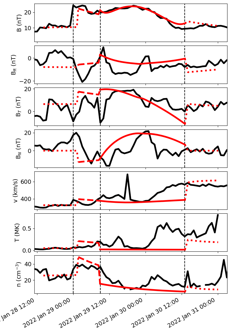 where the B values are in nT, number density in cm-3, velocity in km/s, and temperature in K. -9999 is used as a flag for missing/bad data.
 We note that a ".sats" file shouldn't be used for only a single satellite. Instead the satellite lat, lon, r, and rot can be passed as keywords in the ".txt" file. Instead of using an orbital speed, the trajectory file can be passed via the satPath keyword (instead of ".sats"). The in situ data can be passed via ObsDataFile and the observed boundaries obsShstart, obsFRstart, obsFRend. An example of this is in 20220126.txt, which was used in a previous version of the demo.
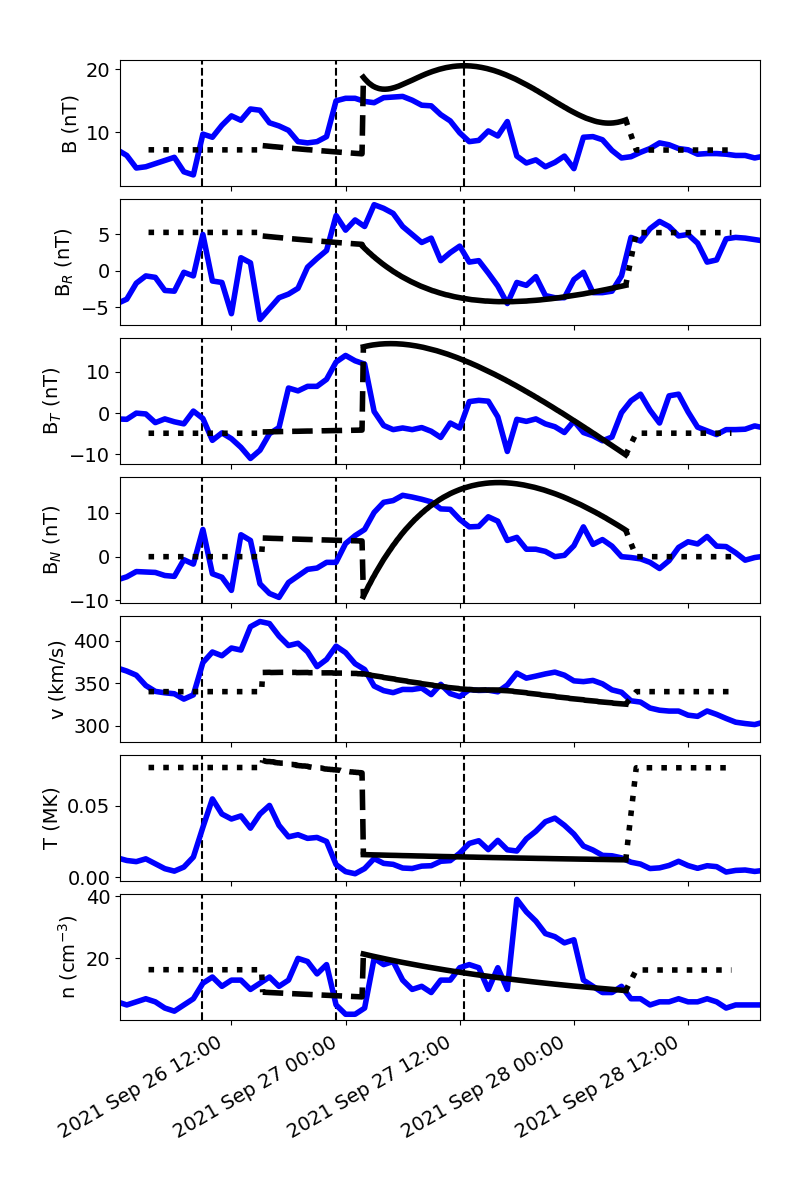
Run the example and the processing script. The results will now appear in the folder 20210923 and are generally the same as what we have already seen. The main difference is in the in situ figures, which are now shown with real dates on the x-axis, as opposed to arbitrary time. The black line showing the OSPREI results (background solar wind, sheath, flux rope) is in the same format as before but now we have a blue line showing the provided observations. The vertical dashed lines indicate the observed boundaries. Note that we are just demoing features here, these are not scientific results or our best attempt simulation of this event and a perfect identification of the observed boundaries.